This notebook is based on the exercises in the Anaconda training Getting started with AI and ML.
I’m copying my notes here as a more in-depth test of the ability to publish directly from Jupyter notebooks, and also to put my notes somewhere I can access them later!
Linear Regression
The most commonly used supervised machine learning algorithm.
This module covered:
- Fit a line to data
- Measure loss with residuals and sum of squares
- Use `scikit-learn`` to fit a linear regression
- Evaluate a linear regression using R2 and train-test splits
Advantages
- simple to understand and interpret
- doesn’t over-fit
When is Linear Regression suitable?
- variables are continuous, not binary or categorical (use logistic regression for the latter)
- input variables follow a Gaussian (bell curve) distribution
- input variables are relevant to the output variables and not highly correlated with each other (collinearity)
Simple Linear Regression
ML often splits into two tasks - regression (predict quantity) and classification (predict a category)
E.g $y = mx+b$
Challenge is to define m and b for “best fit”
Multiple linear regression
With multiple independent variables
e.g. $y = \beta_0 + \beta_1x_1 + \beta_2x_2 + \epsilon$
$\epsilon $ is error due to noise
Multiple variables can get complex, important to use tools to help select only input variables correlated with the output variables.
e.g.:
- Pearson correlation and $R^2$
- adjusted $R^2$
- Akakike Information Criterion
- Ridge and lasso regression
#furtherlearning
Residuals
Residuals are the difference between the data points and the equivalent regression. Linear Regression models aim to minimise the regressions by optimising a loss function such as Sum of Squares.
Overfitting
When ML model works well with training data but fails to predict correctly with new data. Linear regression tends to show low variance and high bias, so less likely to be overfitted. (define terms variance and bias)
Train/Test Splits
Common technique to mitigate overfitting is the use of train/test splits. Training data is used to fit the model, then test data is used to test it with previously-unseen data, if necessary the model can then be tweaked.
Evaluating the model with $R^2$
$R^2$ (the coefficient of determination) ratios the average y-value to the average of the residuals.
It measures how well the independent variables explain a dependent variable, with 0.0 meaning no connection and 1.0 meaning a perfect explanation.
Example using scikit-learn
The package scikit-learn contains many tools to support Machine LEarning techniquies such as Linear Regression.
This worked example demonstrates some of them.
First we import the packages we are going to use, making use of two key utilities from scikit-learn:
train_test_splitmakes it easy to split a set of data into training and test subsets.LinearRegressionfits a linear model with coefficients w = (w1, …, wp) to minimize the residual sum of squares between the observed targets in the dataset, and the targets predicted by the linear approximation.
import pandas as pd
from sklearn.linear_model import LinearRegression
from sklearn.model_selection import train_test_split
We need to import our data into a pandas DataFrame. For convenience I am using one of the datasets provided by the course author
# Load the data
df = pd.read_csv('https://bit.ly/3pBKSuN', delimiter=",")
df
| x | y | |
|---|---|---|
| 0 | 1 | -13.115843 |
| 1 | 2 | 25.806547 |
| 2 | 3 | -5.017285 |
| 3 | 4 | 20.256415 |
| 4 | 5 | 4.075003 |
| 5 | 6 | -3.530260 |
| 6 | 7 | 24.045999 |
| 7 | 8 | 22.112566 |
| 8 | 9 | 5.968591 |
| 9 | 10 | 43.392339 |
| 10 | 11 | 32.224643 |
| 11 | 12 | 14.666142 |
| 12 | 13 | 17.966141 |
| 13 | 14 | -2.754718 |
| 14 | 15 | 25.156840 |
| 15 | 16 | 20.182870 |
| 16 | 17 | 22.281929 |
| 17 | 18 | 16.757447 |
| 18 | 19 | 54.219575 |
| 19 | 20 | 60.564151 |
We need to split our data into inputs and the associated outputs
# Extract input variables (all rows, all columns but last column)
X = df.values[:, :-1]

# Extract output column (all rows, last column)
Y = df.values[:, -1]
We then need to create separate training and testing data to evaluate performance and reduce overfitting.
Her ewe make use of the train_test_split utility.
X_train, X_test, Y_train, Y_test = train_test_split(X, Y, test_size=1.0/3.0, random_state=10)
Next:
- we train the standard
LinearRegressionmodel provided byscikit-learnagainst our training data - then we use the trained model to fit a regression to our test data
The utility allows us to easily score the model using $R^2$.
model = LinearRegression()
model.fit(X_train, Y_train)
result = model.score(X_test, Y_test)
print("R^2: %.3f" % result)
R^2: 0.182
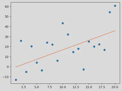
Using matplotlib we can visualise the model output against the whole input data set
import matplotlib.pyplot as plt

plt.plot(X, Y, 'o') # scatterplot
plt.plot(X, model.coef_.flatten()*X+model.intercept_.flatten()) # line
plt.show()